etwfe
Extended Two-Way Fixed Effects for Python — implementing Wooldridge's modern approach to difference-in-differences with staggered treatment adoption.
Two-way fixed effects (TWFE) regressions are widely used for causal inference with panel data, but naive TWFE specifications produce misleading estimates when treatment adoption is staggered and effects vary across cohorts or time. Wooldridge (2023, 2025) proposed a clean solution: fully interact treatment status with cohort and time indicators. This saturated specification—extended TWFE (ETWFE)—recovers cohort-time-specific effects that can be aggregated into interpretable summaries like overall average effects or dynamic event studies.
This Python package development was inspired by the excellent etwfe R package developed by Grant McDermott. It handles the tedious work of building the saturated interaction specification, performs estimation through high-dimensional fixed effects or quasi-MLE, and extracts interpretable treatment effect estimates with proper standard errors.
Installation
pip install etwfeRequires Python 3.8+. Dependencies install automatically.
Sample Data
The examples in this guide use mpdta, a panel dataset tracking teen employment in 500 U.S. counties from 2003 through 2007. Some counties implemented minimum wage increases in 2004, 2006, or 2007, while others never raised their minimum wage—creating a textbook staggered adoption design for difference-in-differences analysis.
from etwfe import etwfe
import pyreadr

# Retrieve the dataset
url = "https://github.com/bcallaway11/did/raw/master/data/mpdta.rda"
pyreadr.download_file(url, "mpdta.rda")
mpdta = pyreadr.read_r("mpdta.rda")["mpdta"]

# Set up the variables
mpdta["first_treat"] = mpdta["first.treat"].astype(int)
mpdta["year"] = mpdta["year"].astype(int)
mpdta["countyreal"] = mpdta["countyreal"].astype(int)

mpdta.head()year countyreal lpop lemp first.treat treat first_treat 866 2003 8001 5.896761 8.461469 2007 1 2007 841 2004 8001 5.896761 8.336870 2007 1 2007 842 2005 8001 5.896761 8.340217 2007 1 2007 819 2006 8001 5.896761 8.378161 2007 1 2007 827 2007 8001 5.896761 8.487352 2007 1 2007
The outcome of interest is lemp, which records log teen employment. The first_treat column indicates the year a county first saw a minimum wage increase (with 0 denoting counties that never experienced an increase). We also have lpop (log population) available as a potential covariate.
Core Workflow
Analysis with etwfe proceeds in two stages. First, etwfe() fits the saturated interaction specification. Second, emfx() transforms the many coefficient estimates into meaningful treatment effect summaries.
Fitting the Model
The etwfe() function requires a formula identifying the outcome and any covariates, plus arguments specifying the time period variable, treatment cohort variable, and the data. Clustering standard errors by unit is generally advisable for panel data.
mod = etwfe(
    fml="lemp ~ lpop",          # outcome ~ covariates
    tvar="year",                # time period
    gvar="first_treat",         # treatment cohort
    data=mpdta,
    vcov={"CRV1": "countyreal"}  # cluster by county
)
Behind the scenes, the function constructs treatment indicators and fully interacts them with cohort and time dummies. The fitted object wraps a pyfixest regression, so methods like .summary() work as expected. However, the raw interaction coefficients lack direct interpretation—that's where emfx() becomes essential.
Extracting Treatment Effects
The emfx() method aggregates the interaction coefficients into interpretable treatment effect estimates. A basic call produces the overall average treatment effect on the treated:
# Overall average effect
mod.emfx()_Dtreat estimate std.error conf.low conf.high 0 1.0 -0.050627 0.012497 -0.075122 -0.026132
The estimate of −0.051 implies that minimum wage increases lowered teen employment by roughly 5% on average across treated counties and post-treatment periods. The confidence interval excludes zero, indicating statistical significance.
The type parameter controls how effects are broken down. Setting type="event" generates an event study that tracks effects relative to treatment timing:
# Dynamic event study
mod.emfx(type="event")event estimate std.error conf.low conf.high 0 0 -0.033212 0.013366 -0.059409 -0.007015 1 1 -0.057346 0.017150 -0.090959 -0.023732 2 2 -0.137870 0.030788 -0.198216 -0.077525 3 3 -0.109539 0.032315 -0.172877 -0.046202
The event study uncovers interesting dynamics: effects begin modestly (−3.3% at the treatment date) but amplify substantially over subsequent years, peaking at −13.8% two years after adoption before moderating slightly.
Creating Visualizations
Event Study Plots
The plot() method generates ready-to-use visualizations. The default style shows point estimates with error bars:
mod.plot(type="event")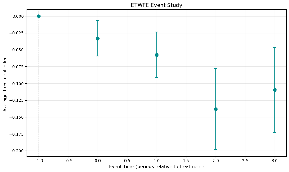
Event study showing treatment effects relative to adoption timing
When using the default cgroup="notyet" control group, pre-treatment coefficients are mechanically zero because not-yet-treated observations serve as controls during those periods. To assess whether parallel trends held before treatment—a crucial diagnostic—restrict the comparison group to never-treated units:
mod_never = etwfe(
    fml="lemp ~ lpop",
    tvar="year",
    gvar="first_treat",
    data=mpdta,
    cgroup="never",              # only never-treated as controls
    vcov={"CRV1": "countyreal"}
)

# Include pre-treatment periods
mod_never.emfx(type="event", post_only=False)event estimate std.error conf.low conf.high 0 -4 0.006896 0.024689 -0.041495 0.055287 1 -3 0.027595 0.018148 -0.007976 0.063166 2 -2 0.023465 0.014531 -0.005017 0.051947 3 -1 0.000000 0.000000 0.000000 0.000000 4 0 -0.021147 0.011394 -0.043478 0.001185 5 1 -0.053356 0.015774 -0.084274 -0.022438 6 2 -0.141080 0.032289 -0.204367 -0.077793 7 3 -0.107544 0.032923 -0.172074 -0.043015
The pre-treatment estimates (events −4 through −2) cluster near zero with confidence intervals spanning it, supporting the parallel trends assumption. For a smoother visual, use ribbon-style confidence bands:
mod_never.plot(type="event", post_only=False, style="ribbon")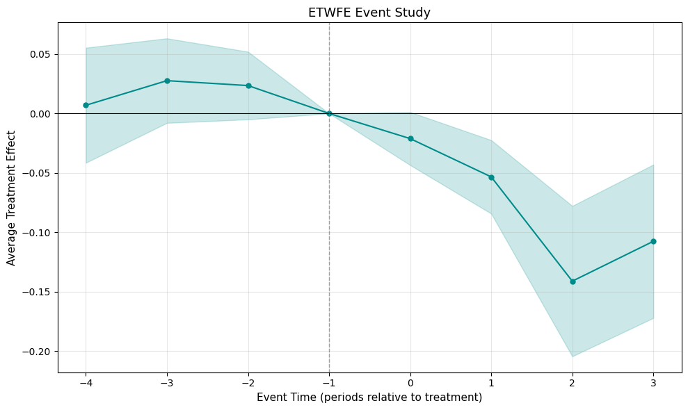
Event study with ribbon-style confidence bands
Comparing Control Group Specifications
You can compare estimates across control group specifications using a regression table format:
import pandas as pd
import numpy as np

# Get event study results
es_never = mod_never.emfx(type="event", post_only=False)[["event", "estimate", "std.error"]]
es_notyet = mod.emfx(type="event")[["event", "estimate", "std.error"]]

# Rename columns
es_never.columns = ["event", "est_1", "se_1"]
es_notyet.columns = ["event", "est_2", "se_2"]

# Merge
table = es_never.merge(es_notyet, on="event", how="outer")
table = table.sort_values("event").reset_index(drop=True)

# Get model stats
nobs_1 = mod_never.model_._N
nobs_2 = mod.model_._N
r2_1 = mod_never.model_._r2
r2_2 = mod.model_._r2
rmse_1 = mod_never.model_._rmse
rmse_2 = mod.model_._rmse

# Function to add significance stars
def add_stars(est, se):
    if pd.isna(est) or pd.isna(se) or se == 0:
        return f"{est:.3f}" if pd.notna(est) else ""
    t = abs(est / se)
    if t > 3.291:
        return f"{est:.3f}***"
    elif t > 2.576:
        return f"{est:.3f}**"
    elif t > 1.96:
        return f"{est:.3f}*"
    elif t > 1.645:
        return f"{est:.3f}+"
    else:
        return f"{est:.3f}"

# Build formatted output
print("\n" + "="*50)
print("                    Event Study")
print("="*50)
print(f"{'':30} {'(1)':>10} {'(2)':>10}")
print("-"*50)

for _, r in table.iterrows():
    evt = int(r["event"])
    label = f"Years post treatment = {evt}"

    col1 = add_stars(r["est_1"], r["se_1"]) if pd.notna(r["est_1"]) else ""
    col2 = add_stars(r["est_2"], r["se_2"]) if pd.notna(r["est_2"]) else ""

    print(f"{label:30} {col1:>10} {col2:>10}")

    se1 = f"({r['se_1']:.3f})" if pd.notna(r['se_1']) and r['se_1'] != 0 else ""
    se2 = f"({r['se_2']:.3f})" if pd.notna(r['se_2']) else ""

    print(f"{'':30} {se1:>10} {se2:>10}")

print("-"*50)
print(f"{'Num.Obs.':30} {nobs_1:>10} {nobs_2:>10}")
print(f"{'R2':30} {r2_1:>10.3f} {r2_2:>10.3f}")
print(f"{'RMSE':30} {rmse_1:>10.3f} {rmse_2:>10.3f}")
print(f"{'FE..first.treat':30} {'X':>10} {'X':>10}")
print(f"{'FE..year':30} {'X':>10} {'X':>10}")
print("-"*50)
print("+ p < 0.1, * p < 0.05, ** p < 0.01, *** p < 0.001")
print("Std. errors are clustered at the county level")
print("="*50)==================================================
Event Study
==================================================
(1) (2)
--------------------------------------------------
Years post treatment = -4 0.007
(0.025)
Years post treatment = -3 0.028
(0.018)
Years post treatment = -2 0.023
(0.015)
Years post treatment = -1 0.000
Years post treatment = 0 -0.021+ -0.033*
(0.011) (0.013)
Years post treatment = 1 -0.053*** -0.057***
(0.016) (0.017)
Years post treatment = 2 -0.141*** -0.138***
(0.032) (0.031)
Years post treatment = 3 -0.108** -0.110***
(0.033) (0.032)
--------------------------------------------------
Num.Obs. 2500 2500
R2 0.873 0.873
RMSE 0.537 0.537
FE..first.treat X X
FE..year X X
--------------------------------------------------
+ p < 0.1, * p < 0.05, ** p < 0.01, *** p < 0.001
Std. errors are clustered at the county level
==================================================
Column (1) uses never-treated controls (cgroup="never") while column (2) uses not-yet-treated controls (cgroup="notyet"). The pre-treatment coefficients in column (1) support the parallel trends assumption. Post-treatment estimates are similar across specifications, with the largest effects occurring at event time 2.
mod_never.plot(type="event", post_only=False)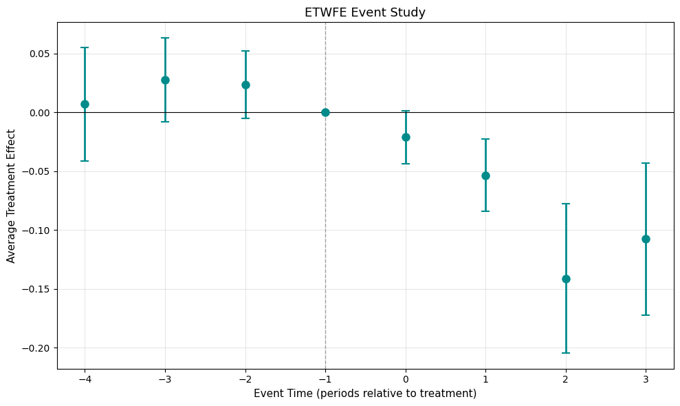
Event study with pre-treatment periods showing parallel trends validation
Effect Heterogeneity
Treatment effects frequently differ across subpopulations. The xvar parameter enables estimation of heterogeneous effects by interacting treatment with a categorical moderator.
As an illustration, we can test whether minimum wage impacts differ between Great Lakes states and other regions:
# Flag Great Lakes states by FIPS code
great_lakes = [17, 18, 26, 27, 36, 39, 42, 55]
mpdta["gls"] = mpdta["countyreal"].astype(str).str[:2].astype(int).isin(great_lakes)
With xvar specified, emfx(by_xvar=True) produces separate estimates for each subgroup:
hmod = etwfe(
    fml="lemp ~ lpop",
    tvar="year",
    gvar="first_treat",
    data=mpdta,
    cgroup="never",
    xvar="gls",                  # heterogeneity dimension
    vcov={"CRV1": "countyreal"}
)

# Subgroup-specific effects
hmod.emfx(by_xvar=True)estimate std.error conf.low conf.high _Dtreat gls 0 -0.051920 0.034637 -0.119809 0.015969 1.0 False 1 -0.039396 0.024296 -0.087016 0.008223 1.0 True
Both regions exhibit negative point estimates, though the confidence intervals overlap considerably—the regional difference doesn't appear statistically meaningful. Visualize the heterogeneous event study with:
hmod.plot(type="event", by_xvar=True, post_only=False, style="ribbon")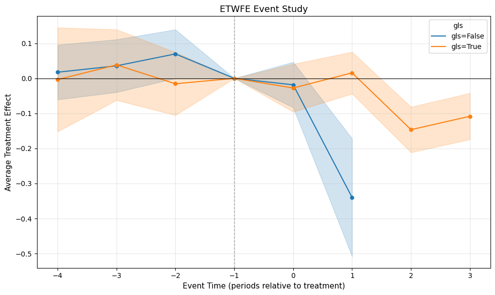
Heterogeneous treatment effects by region (Great Lakes vs. Other)
Nonlinear Specifications
Standard ETWFE presumes that treated and control groups follow parallel trajectories in outcome levels. This "linear parallel trends" assumption becomes questionable when outcomes have bounded ranges or skewed distributions.
When Linear Assumptions Strain
Consider binary outcomes where baseline rates differ markedly between groups—say 15% versus 40%. Expecting parallel evolution in probability levels may be implausible; perhaps trends should be parallel in log-odds instead. Analogous concerns arise with count data clustering near zero, or fractional responses constrained between 0 and 1.
Wooldridge (2023) developed nonlinear ETWFE estimators that assume parallel trends in an index (the linear predictor) rather than the outcome itself. For binary outcomes, this suggests logit; for counts, Poisson. These estimators preserve the same equivalence results as linear ETWFE—pooled quasi-MLE and imputation yield identical estimates.
Poisson Implementation
Here we apply Poisson regression to employment counts rather than log employment:
import numpy as np

# Convert to levels
mpdta["emp"] = np.exp(mpdta["lemp"])

# Poisson ETWFE
mod_pois = etwfe(
    fml="emp ~ lpop",
    tvar="year",
    gvar="first_treat",
    data=mpdta,
    vcov={"CRV1": "countyreal"},
    family="poisson"
)

mod_pois.emfx(type="event")event estimate std.error conf.low conf.high 0 0 -25.349748 15.886320 -56.486936 5.787439 1 1 1.091751 40.295264 -77.886967 80.070469 2 2 -75.124632 23.154168 -120.506802 -29.742462 3 3 -101.823979 27.087814 -154.916095 -48.731864
Robustness Assessment
Even when linear parallel trends seems reasonable, running both linear and nonlinear models provides a valuable robustness check. When estimates align across specifications, confidence in the findings grows. When they diverge, it signals sensitivity to the functional form assumption—useful diagnostic information for interpreting results.
Computational Efficiency
Model fitting via etwfe() runs quickly. The emfx() marginal effects calculation can slow down with large datasets due to the high dimensionality of interaction terms. Two strategies help manage computation time.
Omitting Standard Errors
Setting vcov=False skips variance-covariance estimation, which often dominates runtime. This returns point estimates only—useful for checking specifications before investing in full computation:
# Point estimates without standard errors
mod.emfx(type="event", vcov=False)
Data Compression
The compress=True option implements the data compression approach from Wong et al. (2021). The core insight is that for linear models, data can be reduced to sufficient statistics—aggregated summaries preserving all information needed for estimation.
Compression can shrink datasets with millions of observations to much smaller structures, enabling interactive analysis that would otherwise demand specialized infrastructure. Point estimates match uncompressed results exactly, while standard errors are approximate but typically accurate to 2-3 decimal places.
# Compressed estimation
mod.emfx(type="event", compress=True)
Practical Approach
For large datasets, a staged approach works well:
- Run
emfx(vcov=False)to verify point estimates look sensible - Run
emfx(vcov=False, compress=True)to confirm compression preserves estimates - If results align, run
emfx(compress=True)for approximate standard errors
API Reference
etwfe()
Fit an Extended Two-Way Fixed Effects model.
| Argument | Type | Description |
|---|---|---|
| fml | str | Model formula: "outcome ~ covariates" or "outcome ~ 0" for no covariates |
| tvar | str | Name of the time period variable |
| gvar | str | Name of the treatment cohort variable (period of first treatment; 0 = never treated) |
| data | DataFrame | Panel dataset containing all required variables |
| ivar | str | Unit identifier for unit-level fixed effects (optional) |
| xvar | str | Variable for heterogeneous treatment effects (optional) |
| tref | int | Reference time period (optional; defaults to earliest) |
| gref | int | Reference cohort (optional; defaults to 0 / never-treated) |
| cgroup | str | Control group: "notyet" (default) or "never" |
| fe | str | Fixed effects: "vs", "feo" (default), or "none" |
| family | str | GLM family: "poisson", "logit", "probit", etc. |
| vcov | str | dict | Variance estimator, e.g., {"CRV1": "cluster_var"} |
model.emfx()
Calculate aggregated marginal effects (treatment effect estimates).
| Argument | Type | Description |
|---|---|---|
| type | str | Aggregation: "simple" (overall ATT), "event", "group", or "calendar" |
| by_xvar | bool | Report separate effects by xvar levels (default False) |
| post_only | bool | Restrict to post-treatment periods only (default True) |
| compress | bool | Apply data compression for speed (default False) |
| vcov | bool | Calculate standard errors; set False to skip (default True) |
| predict | str | Prediction scale: "response" (default) or "link" |
model.plot()
Generate visualizations of treatment effects.
| Argument | Type | Description |
|---|---|---|
| type | str | Plot type: "event", "group", or "calendar" |
| style | str | Visual style: "errorbar" (default) or "ribbon" |
| post_only | bool | Display only post-treatment periods |
| by_xvar | bool | Draw separate series for each xvar group |
| figsize | tuple | Figure dimensions as (width, height) |
| color | str | Color for single-group plots |
| colors | list | Color sequence for multi-group plots |
Requirements
- Python >= 3.9
- numpy >= 1.21.0
- pandas >= 1.3.0
- matplotlib >= 3.4.0
- pyfixest >= 0.18.0
References
Wooldridge, J. M. (2025). Two-way fixed effects, the two-way Mundlak regression, and difference-in-differences estimators. Empirical Economics, 69(5), 2545-2587.
Wooldridge, J. M. (2023). Simple approaches to nonlinear difference-in-differences with panel data. The Econometrics Journal, 26(3), C31-C66.
Callaway, B. and Sant'Anna, P. H. (2021). Difference-in-differences with multiple time periods. Journal of Econometrics, 225(2), 200-230.
Wong, J., Forsell, E., Lewis, R., Mao, T., and Wardrop, M. (2021). You only compress once: Optimal data compression for estimating linear models. arXiv:2102.11297.
Acknowledgments
This package relies on several high-quality open-source projects. Estimation uses pyfixest for high-dimensional fixed effects regression. The API and methodology draw heavily from Grant McDermott's etwfe package for R. We thank the developers of these projects for their contributions to accessible econometric software.